Find and highlight Duplicate Cells in Excel
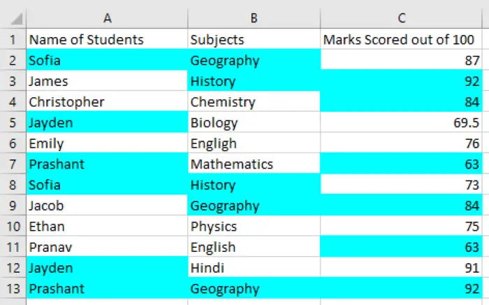
By using the Highlight Cells Rules, you can highlight duplicate cells in your Excel worksheet to avoid confusion and mistakes. The steps to highlight the duplicate cells in an Excel worksheet are listed below: Open the Excel worksheet in which you want to find and highlight the duplicate cells. I have created sample data of marks scored by 10 students in different subjects. Now, you have to select the rows and the columns, the duplicate cells of which you want to highlight. After that, click on Home and go to “Conditional Formatting > Highlight Cells Rules > Duplicate Values.” This will open a new popup window.
In the popup window, you can select different types of highlighting options, by clicking on the drop-down menu. For example, you can highlight the duplicate cells with red, yellow, and green colors, etc. Moreover, if you do not want to fill the entire cells with color, you can highlight their borders or texts only. A custom format option is also available there, which you can select to highlight the duplicate cells with your favorite color. When you are done, click OK. After that, Excel will highlight all the duplicate cells in the selected rows and columns.
If you want to revert the changes, follow the below-listed procedure: If you select the “Clear Rules from Entire Sheet” option, it will clear the highlighted cells from the entire Excel sheet. That’s it. Related posts:
How to delete duplicate rows in Excel and Google Sheets.How to calculate Compound Interest in Excel.